
Solving the Transportation Problem
A beginner-friendly tutorial that covers BFS, MODI, degeneracy and full iterations.

Introduction
What is the Transportation Problem
The Transportation Problem (TP) is a classic optimization model in Operations Research that determines the most cost-efficient way to move goods from multiple sources (e.g., factories, plants, warehouses) to multiple destinations (e.g., markets, retail centres, customers).
You are given:
A set of m supply points (each with a fixed supply)
A set of n demand points (each with a required demand)
A cost matrix that specifies the unit shipping cost from every supply point to every demand point
The goal is simple:
Allocate shipments from each source to each destination in a way that meets all supply and demand at the minimum possible total cost.
Formally, TP is a special case of a linear programming problem where:
All constraints are equalities (supply and demand)
All variables are non-negative
Most importantly: the constraint matrix is highly structured, allowing faster, specialized solution methods.
In simple terms:
TP tells you the cheapest way to transport something from where it is produced to where it is needed.
Where OR uses it
The Transportation Problem appears in numerous real-world applications, such as:
1. Logistics & Distribution
Shipping goods from factories to regional warehouses
Moving inventory across a multi-echelon supply chain
Deciding distribution for FMCG, pharma, electronics
Optimising milk runs and distribution centres
2. Manufacturing
Allocating raw materials to plants
Assigning components to assembly units
Minimising material-handling costs
3. Retail & E-commerce
Order fulfillment optimization
Routing goods from dark stores to delivery hubs
Optimal hub-and-spoke logistics planning
4. Agriculture & Food Supply Chains
Transport of grains, fruits, vegetables
Reducing spoilage by optimal routing
5. Energy and Steel Sectors
Coal → power plants
Steel billets → rolling mills
Petroleum transport → depots
Why this method remains important
Even though modern solvers like CPLEX, Gurobi, and SciPy can solve LPs instantly, the Transportation Problem remains vital for three reasons:
1. Transparency and Managerial Insight
Unlike black-box solvers:
BFS methods (Northwest Corner, Least Cost, Vogel’s)
Optimization methods (MODI / U–V method)
…show why a route is optimal.
Managers and students can understand:
Why some routes are used over others
Which supply/demand constraints are binding
Why costs reduce after each iteration
How changes in capacity affect cost
2. Large-Scale Practical Use
Many industries still code customized transportation solvers because:
Data structures match their operational tables
Special algorithms run faster than general LP solvers
TP models often recur daily (dynamic supply chains)
Even large companies like Amazon, Flipkart, FedEx, Marico, HUL, and Tata Steel use modified TP logic inside their logistics planning systems.
3. Foundation for Advanced OR Concepts
TP is the gateway to:
Network optimization
Minimum cost flow
Assignment problems
Supply chain simulation
Transshipment
Vehicle routing and TSP variants
Students who understand TP deeply can learn these faster.
1. The Problem Setup
Before we learn how to solve the Transportation Problem, we need to understand the basic components that define it. These elements form the foundation for every method you will see later: BFS, Least Cost, Vogel’s Approximation, and the MODI / U–V optimization technique.
1.1 Supply, Demand, and Cost
Every transportation problem has three essential inputs:
Supply (at each source)
Each source (factory, plant, warehouse) has a fixed quantity available for shipping.
Examples:
Factory A → 40 units
Factory B → 25 units
Warehouse C → 35 units
This quantity cannot be exceeded.
Demand (at each destination)
Each destination (market, customer zone, depot) requires a certain quantity.
Examples:
Market X → 20 units
Market Y → 30 units
Market Z → 50 units
Demand must be fully met.
Cost (per unit shipped)
For every pair (source i → destination j), there is a per-unit shipping cost, often coming from:
freight charges
distance × fuel cost
tolls
handling or packaging
contractual rates
This forms the cost matrix.
Example cost matrix (just conceptual):
               Destinations
                X   Y   Z
              -------------
            A   4   6   8
   Sources  B   5   3   7
            C   9   5   2
              -------------
Reading the cost matrix is simple: the cost of shipping from C to Z is 2 per unit.
1.2 The Transportation Tableau
The transportation tableau is the tabular representation that we use to work through the BFS and MODI methods.
It contains:
rows → supply points
columns → demand points
cells → shipping cost
rightmost column → supply values
bottom row → demand values
bottom-right → a check cell (not used)
Example (illustrative):
               Destinations
                 X   Y   Z  | Supply
           -------------------------
            A |  4   6   8  | 40
   Sources  B |  5   3   7  | 25
            C |  9   5   2  | 35
           -------------------------
       Demand | 20  30  50
The tableau helps visualize:
allocations
unfilled cells
degeneracy
opportunity costs
loops
potentials (u, v)
All the work we’ll do later happens on this table.
1.3 Balanced vs Unbalanced Problems
Balanced Problem
When total supply = total demand
→ A direct BFS can be created.
Example:
Supply: 40 + 25 + 35 = 100
Demand: 20 + 30 + 50 = 100
Balanced
This is the most common case.
Unbalanced Problem
When total supply ≠ total demand
There are two possibilities:
Case 1 — Supply > Demand
Add a dummy destination with demand equal to the excess.
Costs are usually set to zero or a neutral value.
Case 2 — Demand > Supply
Add a dummy source with supply equal to the shortfall.
Costs are again usually zero or neutral.
After adding dummy rows/columns → the problem becomes balanced.
Why do we do this?
Because BFS and MODI rely on a square structure where:
The number of basic variables in any BFS = m + n − 1
This only holds when total supply = total demand.
1.4 Basic Definitions (Used Later)
These terms will be used throughout the tutorial.
1. Basic Feasible Solution (BFS)
An allocation that:
satisfies all supply and demand
uses exactly m + n − 1 allocated cells
contains no loops
This is the starting point for MODI.
2. Degeneracy
When the BFS uses fewer than m + n − 1 allocations.
This causes issues in calculating potentials (u, v) and loops.
Fix by adding a tiny value ε (epsilon) in any empty cell.
3. Cost Coefficient (cᵢⱼ)
The shipping cost from source i to destination j.
4. Allocation (xᵢⱼ)
The number of units shipped along a route.
During BFS, you fill these systematically.
During optimization, these values change.
5. Opportunity Cost (Δᵢⱼ)
Computed during U–V / MODI method.
If Δᵢⱼ < 0 → the route can improve total cost.
This drives pivots and loops.
6. Potentials (uᵢ and vⱼ)
Dual variables associated with rows and columns.
Used to compute opportunity costs:
Δᵢⱼ = uᵢ + vⱼ - cᵢⱼ
These are at the heart of the optimization process.
7. Loop
A closed path formed during optimization to adjust allocations.
Alternating + and − signs help redistribute units without violating row/column totals.
2. A Transportation Problem
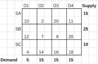
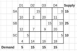
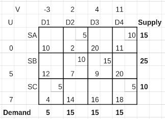
Let us examine a situation of a balanced transportation probem. There are 3 sources from where a good is to be transported to 4 destinations. The cost of transportation is given in the following table.
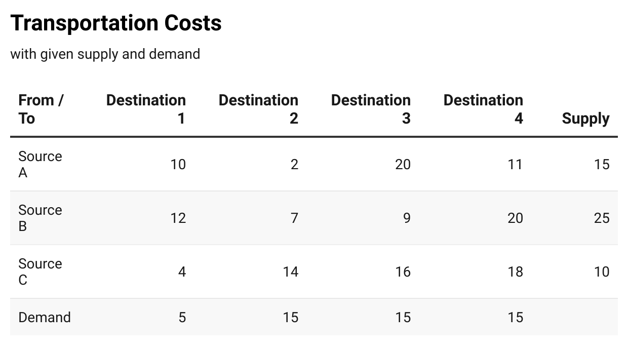
This is a balanced transportation problem. The total demand to be met, 5 + 15 + 15 + 15 = 50 equals the total available supply, 15 + 25 + 10 = 50
The problem is to allocate the supplies from the 3 sources to the 4 destinations such that the cost incurred is the lowest.
Let us develop the linear programming formulation of this problem.
If the total supply is more than the total demand, how does this change? Can we write the LP constraints as
Also, in the most general unbalanced case, can we simply write the constraints as
Solving the Transporation Problem
In other words finding the minimum cost routing for this problem, with the given demand and supplies and the route costs for unit quantity transported.
The initial step is to arrive at a Basic Feasible Solution (BFS) using any one of three methods, viz. (i) North-West Corner Method, (ii) Least Cost Method, and (iii) Vogel Approximation Method or (VAM). We demonstrate all three methods for the given problem.
Please note that, in general, VAM gives the best (lowest cost) initial solution, followed by the Least Cost method and the NW Corner method, in that order.
The final step is to arrive at the Optimal Solution using the MODI (Modified Distribution Method), also known as the UV Method.
Finding BFS: North-West Corner method
As its name suggest this method allocates the maximum amount possible to the NW corner cell, iteratively.
The Cost Matrix, as shown earlier, is reproduced below.

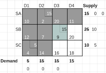
As shown in Iteration 1 below, choosing the NW cell which has a cost of 10 per unit, we allocate 5 units, i.e. minimum of demand, 5 and supply, 15. This leaves 10 units of supply from supplier SA, while the demand from D1 is fulfilled.
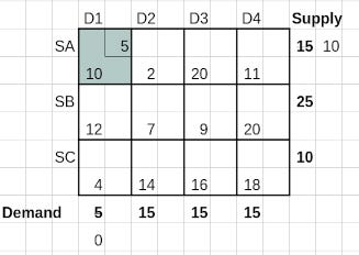
Now, since column 1 corresponding to D1 has its demand exhausted, it is not to be considered for any further allocation. This leaves us with the Iteration 2 table, where we again apply the NW Corner rule to allocate the minimum of 15 and 10 units, i.e. 10 units to cell (SA, D2). This exhausts supplier SA’s supply while D2 is left with a remaining demand of 5 units.
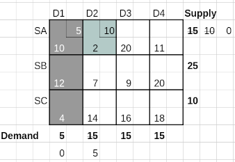
In Iteration 3, we remove row 1 where supply is exhausted, and allocate the lesser of 5 and 25 units to cell (SB, D2) which is the current NW corner in the available matrix of cells. The supply from SB is reduced by 5 to 20, while the demand from D2 is completely satisfied.
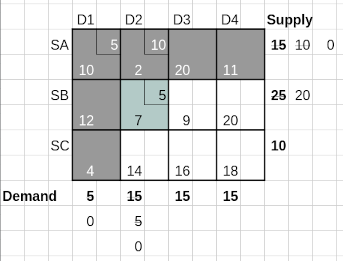
Continuing in this manner, in Iteration 4, we allocate 15 units to the next available NW Corner (SB, D3) in Iteration 4, reducing the corresponding marginal demand and supply.
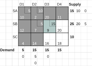
Can we see what happens next? Column 3 is exhausted leaving only the two cells in column 4. Applying the NW Corner rule we allocate 5 units to cell (SB, D4) in Iteration 5 (not shown here), and finally the 10 remaining units to the only remaining cell (SC, D4) in Iteration 6, shown below.
The cost of this Basic Feasible Solution arrived at by the NW Corner Method is obtained by multiplying the allocated quantities (North East) with the cost (South West) for allocated cells. This is 5*10 + 10*2 + 5*7 + 15*9 + 5*20 + 10*18 = 525
Finding BFS: Least Cost method
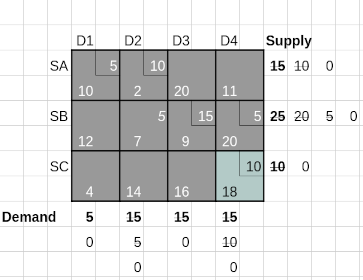
This algorithm is better than the NW Corner method for getting the BFS. Instead of choosing the North-West corner iteratively, in this method we choose the cell having the least cost associated. Tie breaks can be broken randomly.
Let us start from the Cost Matrix, shown earlier. The first allocation is made to the cell with the least cost, viz. (SA, D2). The lesser of the values for demand, 15 and supply, 15 is 15 which is allocated to this cell. This is shown in the Iteration 1 table below.
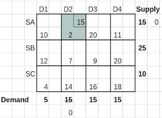
Post the allocation the reduced marginals for supply and demand indicate that both the second column and the first row are out of contention. Iteration 2 shown below, repeats the strategy.
Similarly, Iteration 3 shown below, picks the remaining least cost cell, (SB, D3)
Finally, in Iteration 5 we reach the BFS using the Least Cost Method.
The cost of this Basic Feasible Solution arrived at by the Least Cost Method is obtained by multiplying the allocated quantities (Nort East) with the associated costs (South West) for allocated cells. This is 15*2 + 15*9 + 10*20 + 5*4 + 5*18 = 475
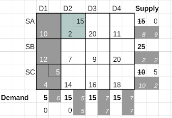
Finding BFS: Vogel’s Approximation Method (VAM)
This method yields the best BFS for a transportation and is a refinement of the Least Cost method. Here, instead of choosing the least cost cell from the cells that are available for allocation, we choose the lowest cost cell from the row or column with the highest penalty. The penalty is computed as the difference between the two lowest costs in the available cells for each row and column.
In this section we go thorough an illustration of Vogel’s Approximation Method for arriving at the BFS using the Cost Matrix shown earlier and reproduced here as well.
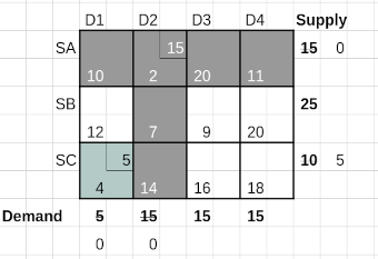
In the following table VAM - Iteration 1, we compute the difference between the two lowest costs for each row and each column. The differences are shown on a gray background. For example for the first row the two lowest values are 10 and 2, resulting in a difference of 8. Similarly for column 3, for example, the difference between the smallest two values, 9 and 16 is 7.
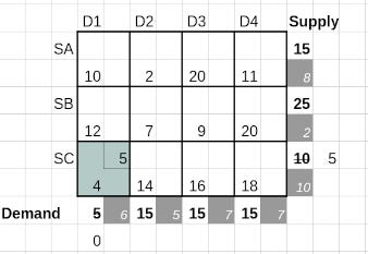
The maximum of these differences, 8, 2 and 10 for the rows and 6, 5, 7 and 7 for the columns is 10. This maximum difference is in the third row, i.e. the row for supplier SC. The minimum cost among all available cells in this row is 4 in cell (SC, D1). This cell is thus earmarked for allocation.
The quantity to be allocated is 5. As in the earlier methods, the smaller of the available supply for that row, 10 and the demand for that column , 5 determines the quantity to be allocated in this cell.
Finally this reduces the supply for SC from 10 to 5 while it completely exhausts the demand from D1, thereby removing column 1 for any future consideration.
Iteration 2 follows similarly with a recomputation of the penalties. The column penalties for columns 2, 3 and 4 remain the same while the row enalties are recomputed since the first column values are not available now.
The maximum penalty is for row SA and the lowest cost is 2 occurring in cell (SA, D2). The corresponding available demand and supply are both 15 - so 15 is allocated to this cell. This exhausts the supply for SA and the demand from D2, removing row 1 and column 2 for any further contention.
This takes us to Iteration 3 of the VAM method shown below.
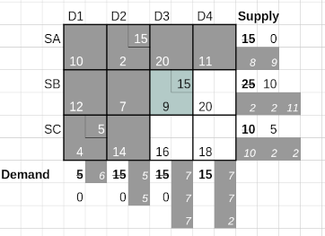
The maximum penalty, 11, now occurs for row SB, which has a lowest available cell cost of 9. This is earmarked for the next allocation of the lower of 25 and 15 - available supply and remaining demand. So 15 is allocated to cell (SB, D3), exhausting the column demand while reducing the row supply from 25 to 10.
Iteration 4 continuing the VAM method is shown below.
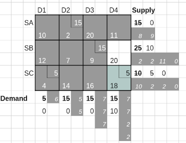
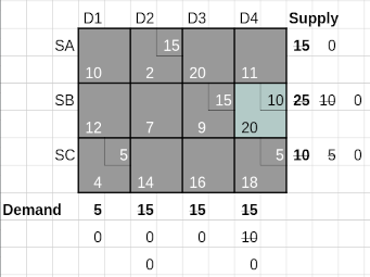
Only one column is available for allocations at this stage. The maximum penalty is 2 and the least cost is 18 for cell (SC, D4). An allocation of the minimum of 10 and 15 units is made to cell (SC, D4). After reducing the available demand to 10 and noting that the supply from SC is exhausted, we arrive at the final iteration that completes the allocations using VAM.
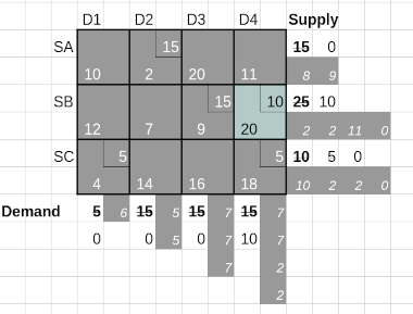
The cost of this Basic Feasible Solution arrived at using the VAM method is obtained by multiplying the allocated quantities (Nort East) with the associated costs (South West) for allocated cells. This is 15*2 + 15*9 + 10*20 + 5*4 + 5*18 = 475, which is the same as what we obtained using the Least Cost method.
Basic Feasible Solution Costs
Using the North West Corner method 525
Using Least Cost method 475
Using Vogel’s Approximation method 475
Is 475 the lowest cost of transportation? We shall find this out in the next section which checks a solution for optimality and if suboptimal uses a method to drive the solution to optimality.
Finding the Optimal Solution - MODI / UV method
The Initial Basic Feasible solution is the starting point for the MODI iterations to reach optimality. In our example, both the Least Cost and VAM give us the same BFS. Below is the allocations we use as the starting point for optimizing the transportation.
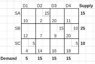
The cost of this transportation is 475 as we have seen earlier.
For a unique solution we need m + n - 1 allocations, where m is the number of rows and n is the number of columns . In our example case m=3 and n=4. So we need 6 allocations for a unique solution.
Here, we have only 5 cell allocations. We thus need a zero allocation in one of the unallocated cells.
The zero allocation has to be made in a cell which does not form a closed loop with other allocated cells. Cell (SB, D1) is not a candidate since a zero allocation in that cell results in a closed loop (SB, D1) → (SB, D4) → (SC, D4) → (SC,D1) → (SB, D1)
We decide to allocate a dummy 0 units to (SA, D1) to have 6 allocations as required. This results in the BFS shown below.
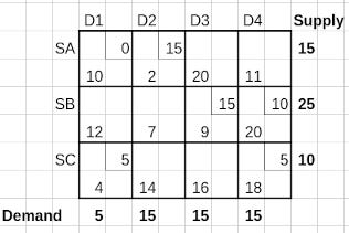
Iteration 1
We now assign U’s as the row potentials or cost levels of each row, and V’s as the column potentials or cost levels of each column.
For every allocated cell (basic cell), the MODI formula holds:
This is used to determine all U’s and V’s as shown below.
We have 6 allocated cells giving rise to 6 equations of the above form, and 7 unknowns - 3 U’s and 4 V’s. We assume one of the U’s or V’s to be zero.
We can always take U₁ as 0.
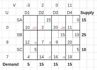
The table with the U’s and V’s is shown below.

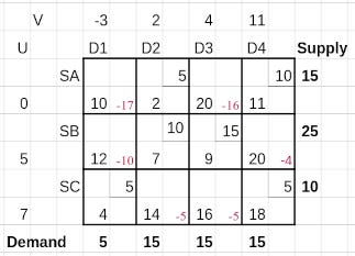
In the next step we use the U’s and V’s to compute opportunity costs (Δ) for each unallocated cell (i, j) using the formula
If all Δ ≤ 0, the solution is optimal.
If any Δ > 0, the most positive indicates where to improve.
The computed Δ values are shown in the South East cornet of each unallocated cell in the table below.
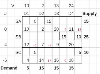
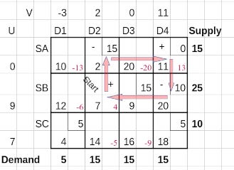
There is only one cell (SA, D4) with a positive value of Δ. So this has to enter the basis set in order to reduce cost of transportation. To decide which cell leaves the basis set in turn, we construct a closed loop starting from the new basis cell and passing through other basis cells using only horizontal and vertical connectors.
Such a closed loop is shown using red arrows in the next table.
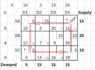
The cells in this route cover 3 basis cells and the new identified basis cell. We start with a positive sign on the new basis cell and assign alternating signs along the cells in the route. Then we choose the minimum allocated value in the negative (-) cells; a minimum of 0 in cell (SA, D1) and 5 in cell (SC, D4). The resulting value, 0 is subtracted from the cells marked with - sign and added to the cells marked with + sign.
Though adding or subtracting zero does not change the allocations it achieves something important. The cell (SA, D1) moves out of the basis set while the new cell (SA, D4) moves in.
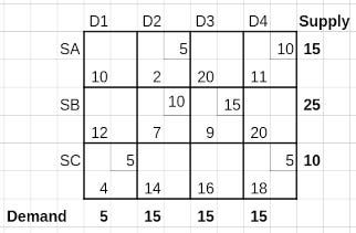
Iteration 2
At the end of iteration 1 we have the following allocations.
In order to assign the U’s and V’s - row column penalties, we take U₁ as 0.
The following equations result in solution of the remaining U’s and V’s.
This gives us the following table, where with the help of the computed U’s and V’s we compute the Δ values (in red) for the unallocated cells.
Cell (SB, D2) with a Δ value of 4 is the only positive Δ value, so this cell enters the basis for the next iteration. A closed loop is constructed now starting from this cell and travelling through other allocated cells.
The route is (SB, D2) → (SA, D2) → (SA, D4) → (SB, D4) → (SB, D2) closing the loop. We start with a positive sign on the new basis cell and assign alternating -/+signs along the cells in the route. The minimum allocations in the negative (-) cells 15 in (SA, D2) and 10 in cell (SB, D4) is 10. This resulting value, 10 is subtracted from the cells marked with - sign and added to the cells marked with + sign giving us the following table as the start of the next iteration.
Iteration 3
Taking U₁ as 0, we derive the remaining U’s and V’s from the following equations.
The table with the U’s and V’s is shown next
. Now the Δs are computed for the unallocated cells.
We see that all unallocated cells have negative Δ values, implying that we have already reached the optimum transportation routing.
The optimum cost is 5*2 + 10*11 + 10*7 + 15*9 + 5*4 + 5*18 = 435
Summary of cost improvements are:
Basic Feasible Solution Costs
Using North West Corner method 525
Using Least Cost method 475
Using Vogel’s Approximation method 475
MODI / UV Optimum Cost 435
Closing Thoughts
The Transportation Algorithm is elegant; small, logical steps solve a large optimization problem efficiently. With a clear BFS, proper u and v assignments, and careful loop adjustments, the method becomes intuitive.
I would love to know if this tutorial was helpful.
This is my first substack post and your comments will help me to make my future posts more engaging and useful.
very well explained. many thanks. Am I correct to say this is foundation for more complicated problem like natural gas scheduling?